“It doesn't make sense to hire smart people and then tell them what to do. We hire smart people so they can tell us what to do.”

Steve Jobs, from Steve Jobs: His Own Words and Wisdom

Basel Committee on Banking Supervision, Consultative Document “Review of the Credit Adjusted Valuation Risk Framework,” July 2015

We open with a well-known but often ignored piece of advice from the legendary Steve Jobs. The second quotation, courtesy of the Basel Committee on Banking Supervision, shows what happens in bank regulation and credit risk management when Steve Jobs’ advice is ignored. In this note, we explain how the modern framework for credit risk management was established by Robert A. Jarrow, Stuart Turnbull, and Kaushik Amin in three key articles during the 1992 through 1995 period. If this now 25-year framework is intelligently applied, the proper valuation formulas for credit-adjusted valuation are both simpler and more accurate than the ad hoc expression for “Kspread” shown above. We use this framework to illustrate the well-established peer-reviewed approach to credit risk that represents best practice in financial economics as of this writing. We contrast that with the ever-changing ad hoc formulas for CVA emerging from Basel when regulators tell smart people what to do without doing their proper homework.

Credit Risk-Adjusted Valuation: The Basics

In this section, we summarize the key results of some classic works in financial theory by Heath, Jarrow and Morton [1992], Amin and Jarrow [1992], Jarrow and Turnbull [1995], Jarrow [2001], and Chava and Jarrow [2004]. While many other famous financial economists have contributed greatly to credit risk research, we focus on these articles in the interest of brevity.

Common sense and solid academic research confirms these essential elements of credit risk-adjusted valuation:

1. The risk-free valuation curve is driven by many random factors. It is not best practice to assume rates are constant or to assume one factor is enough to capture variation in the risk-free curve. Heath, Jarrow and Morton [1992] is the definitive multi-factor work in this regard.

2. The marginal cost of funds to the owner of the defaultable security (we use this term broadly) is irrelevant. The price of the defaultable security depends on the interaction of many market participants who most likely agree on only one yield curve: the risk-free curve. Bankers and bank regulators, used to the funds transfer pricing concept in bank interest rate risk management, share the blame for assuming that the bank’s cost of funds drives the pricing on the debt of a risky borrower. If the bank were a monopolist, that may be true, but that’s not the case. Nowhere in a respected financial journal is the funding yield curve of the owner of a defaultable security used in valuation. Jarrow and Turnbull [1995] provide the original valuation framework for valuing risky debt in a multi-factor random interest rate environment.

3. Many macro-economic factors vary randomly and securities based upon these macro factors are often traded in the market place. Amin and Jarrow [1992] explain how these traded macro-factor-related securities are priced.

4. The default probability of the debt issuer varies randomly over time as a function of the risk-free yield curve, macro factors, and idiosyncratic incidents that are unique to the issuer. Jarrow [2001] expands on Jarrow and Turnbull [1995] in this regard.

5. The recovery rate, conditional on default, varies randomly also as a function of a similar, overlapping list of macro factors. This causes the often-observed correlation between default probabilities and loss given default, defined as one minus the recovery rate expressed as a percent of a bond’s par value.

6. The interaction of all of these factors impacts the price of the defaultable security in a straightforward way, as explained in Jarrow [2013].

Credit Spreads: Putting the Cart Before the Horse

In a recent paper, van Deventer and Sankaran [2016] explained the model risk in using credit spreads to derive bond prices because of the large number of false assumptions underlying the credit spread assumption. The proper procedure is to use the approach we demonstrate below to value the credit risky security, and then, given the price, the credit spread is known with certainty. Van Deventer and Sankaran used bond prices from Lehman Brothers on September 15, 2008 to illustrate the problems with the calculation assumptions used to derive spreads:

1. “The corporate bond will pay its full principal amount (this argument is false: the bond is defaulting and will pay its recovery value). In the Lehman case, the average bond price is 33.80, with a relatively small standard deviation of 1.60 over the 22 bond issues. If we say that the recovery amount is roughly 33.80, the assumption that the bond will pay 100 is grossly wrong and overstated.

2. “The full principal amount will be paid at maturity (false: the recovery amount will be paid upon resolution of bankruptcy proceedings in court. The longest maturity bond from Lehman in the chart above is 2027, but most of the recovery payments to Lehman bond holders have already been made).

3. “All interest coupons will be paid (false: only those interest payments prior to the bankruptcy filing on September 15, 2008 will be paid).

4. “Bonds of different maturities and coupons have different cash flows (false: they have identical cash flows upon default: interest payments are zero and the principal that will be paid is the recovery amount; and the payment date is the date [or series of dates] that recovery payments are made after the bankruptcy is resolved in court).

5. “Credit spreads are constant for all periods prior to maturity of bond k (false, they vary by maturity for firms that are not near bankruptcy).

6. “Credit spreads for bond k are different from bond j if they have different maturities, but these constant spreads are inconsistent from time zero to years to maturity = min(j,k). To give a specific example, the credit spread formula implies that the credit spread is 16.96% for the 2027 bond but 45.23% for the bond due in January 2012. In short, for the period from September 2008 to January 2012, the spread formula implies that the coupons for the 2012 bond have a spread that is almost 30 percentage points higher than the 16.96% spread that applies to coupons covering the same time period on the bond due in 2027. This inconsistency is nonsense.

7. “The risk free yield is constant for all periods until the risk-free bond’s maturity (false, this is a well-known problem with the yield to maturity calculation). Even for the risk free curve, the yield to maturity for bonds of different maturities implies different discount rates during the overlapping period when both bonds are outstanding.”

A Worked Example

Using standard econometrics and statistical procedures, the random factors that drive the risk-free yield curve and macro-economic factors are determined, and their volatility is established.2 Best practice is to allow these factor volatilities to vary depending on the history of the driving factors. For example, higher interest rates usually lead to higher interest rate volatility, subject to a cap for reasons suggested by Heath, Jarrow and Morton [1992]. The parameters are set so that the entire risk-free yield curve is correctly priced. Moreover, all traded securities that depend on macro-economic factors will also be correctly priced.

We consider the case of a derivative security where Bank of America (BAC) is the defaultable counterparty. We assume that the payments owed by Bank of America on the derivative security vary randomly according to still another overlapping set of macro factors. This causes correlation with Bank of America default probabilities, recovery rates, and the discount rates used for valuation. To illustrate the part of the calculation which would be new to many readers, we fit a function which links future Bank of America 3 month default probabilities as a function of macro-economic shocks to the risk free curve, the S&P 500, Brent oil prices, the Case-Shiller 20 City Home Price index, GDP growth and the unemployment rate. The actual annualized 3-month default probabilities are shown as red dots, and the predicted default probabilities are shown as blue dots:

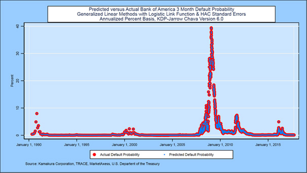
Four points on the risk-free U.S. Treasury yield curve were statistically significant: the idiosyncratic movement of 3 month forward rates with maturities in 6 months, 10 years, 20 years, and 30 years. The statistically significant macro-economic factors were idiosyncratic shocks to the return on the Standard & Poors 500 index, GDP growth, and the unemployment rate.3 The adjusted r-squared of a linear regression linking predicted and actual 3 month default probabilities had an r-squared of 93.45%. Additional details are available from the author. While the example below is too simple to fully exploit the insights of macro-factor drivers of default probabilities, a full enterprise-wide credit valuation adjustment simulation would use hundreds of thousands of scenarios and include each individual credit-risky transaction.4 In actual practice, parameters of the models used would be fitted both to history and to current market prices such that the full risk-free yield curve and traded macro factors would be priced perfectly in a large-scale Monte Carlo simulation.

A simple table showing the payoffs according to five major scenarios, all of which are subject to a default/no default sub-scenario, is given here:

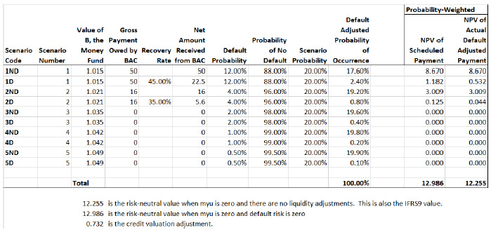
The scenarios are labeled 1ND (first scenario, no default), 1D (first scenario, default) and so on. The gross payment owned by Bank of America on the derivative, the recovery rate, and the default probability of Bank of America are all dependent on the simulated risk-free yield curve and relevant macro factors in each of the 5 scenarios. The probability of each major scenario, using typical Monte Carlo simulation procedures, is equal for all five scenarios at 20%. The probability is modified by multiplying the (random) probabilities of default/no default in each macro scenario. The probability of cash flow in scenario 1ND is 20% x 88%, or 17.60%. The probability of cash flow in scenario 1D is 20% x 12%, 2.40%. The total of the probabilities of scenarios 1ND and 1D must be 20%, of course. The total of the probabilities for all of the 10 sub-scenarios must be 100%.

The credit-adjusted amount received from Bank of America, of course, depends on whether the Bank defaults. In scenario 1ND, the full $50 scheduled amount is received. In scenario 1D, only the random recovery rate (45% in this scenario) times the scheduled amount (50) is received, $22.50.

In the last two columns, we discount the scheduled payment by dividing by the simulated future value of $1 invested in the risk-free short-term interest rate until the payment date. In both scenarios 1ND and 1D, this money fund value is 1.015. In the second column from the right-hand side, we discount the scheduled payment and ignore defaults. We weight the discounted present values by their probability and add them together to get a 12.986 value for the derivative security, assuming no credit risk. The right-hand column discounts the amounts net of the impact of default, for a credit-adjusted value of 12.255. The difference between the two values, 0.732, is the credit valuation adjustment, done correctly.

Practical Enterprise Scale Implementation

Before turning to large scale implementation, we owe it to readers with a background in theoretical financial to explain that we prefer to make the assumption that the risk-6 neutral probabilities of default (used in the table) and the empirical probabilities of default (estimated using historical data) are equal. We refer readers to a classic paper by Jarrow, Lando and Yu [2005] for the theoretical justification.

For implementation on a full balance-sheet wide basis, one would use a modern enterprise-wide risk management system5 combined with state of the art “reduced form” default probabilities.6 The credit valuation adjustment for every relevant transaction and the related capital requirements from the credit risk being absorbed would be measured using a single integrated credit-adjusted value-at-risk simulation.

Conclusions

Regulators and accountants have often violated Steve Jobs’ advice when putting together banking regulations and accounting pronouncements. The proper procedures are much more straightforward that the initial quote from the Bank for International Settlements, and they are much easier to implement on a massive scale than the ad hoc BIS procedures.

It is important to remember that both accounting standards and banking regulations set MINIMUM standards, not MAXIMUM standards designed to restrict the maximum accuracy that a firm can achieve.

Check Out : Performance Risk Management